Demonstration of workflow

The methods below are described in our article

Larsson, Held, et al. (2024) Reconstructing the regulatory programs underlying the phenotypic plasticity of neural cancers. Nature Communications 15, 9699 DOI 10.1038/s41467-024-53954-3

Here we demonstrate the scregclust workflow using the PBMC data from 10X Genomics (available here). This is the same data used in an introductory vignette for the Seurat package. We use Seurat for pre-processing of the data.

# Load required packages
library(Seurat)
library(scregclust)

Download the data

We are focusing here on the filtered feature barcode matrix available as an HDF5 file from the website linked above. The data can be downloaded manually or using R.

However you obtain the data, the code below assumes that the HDF5 file containing it is placed in the same folder as this script with the name pbmc_granulocyte_sorted_3k_filtered_feature_bc_matrix.h5.

url <- paste0(
  "https://cf.10xgenomics.com/samples/cell-arc/2.0.0/",
  "pbmc_granulocyte_sorted_3k/",
  "pbmc_granulocyte_sorted_3k_filtered_feature_bc_matrix.h5"
)
data_path <- file.path(
  tempdir(), "pbmc_granulocyte_sorted_3k_filtered_feature_bc_matrix.h5"
)

download.file(url, data_path, cacheOK = FALSE, mode = "wb")

Load the data in Seurat and preprocess

To perform preprocessing use Seurat to load the data. The file ships with two modalities, “Gene Expression” and “Peaks”. We only use the former.

pbmc_data <- Read10X_h5(
  data_path,
  use.names = TRUE,
  unique.features = TRUE
)[["Gene Expression"]]
#> Genome matrix has multiple modalities, returning a list of matrices for this genome

We create a Seurat object and follow the Seurat vignette to subset the cells and features (genes).

pbmc <- CreateSeuratObject(
  counts = pbmc_data, min.cells = 3, min.features = 200
)

pbmc[["percent.mt"]] <- PercentageFeatureSet(pbmc, pattern = "^MT.")
pbmc <- subset(pbmc, subset = percent.mt < 30 & nFeature_RNA < 6000)

SCTransform is used for variance stabilization of the data and Pearson residuals for the 6000 most variable genes are extracted as matrix z.

pbmc <- SCTransform(pbmc, variable.features.n = 6000)
#> Running SCTransform on assay: RNA
#> vst.flavor='v2' set. Using model with fixed slope and excluding poisson genes.
#> Calculating cell attributes from input UMI matrix: log_umi
#> Variance stabilizing transformation of count matrix of size 19168 by 2686
#> Model formula is y ~ log_umi
#> Get Negative Binomial regression parameters per gene
#> Using 2000 genes, 2686 cells
#> Found 6 outliers - those will be ignored in fitting/regularization step
#> Second step: Get residuals using fitted parameters for 19168 genes
#> Computing corrected count matrix for 19168 genes
#> Calculating gene attributes
#> Wall clock passed: Time difference of 14.77731 secs
#> Determine variable features
#> Centering data matrix
#> Place corrected count matrix in counts slot
#> Set default assay to SCT

z <- GetAssayData(pbmc, layer = "scale.data")
dim(z)
#> [1] 6000 2686

Use scregclust for clustering target genes into modules

We then use scregclust_format which extracts gene symbols from the expression matrix and determines which genes are considered regulators. By default, transcription factors are used as regulators. Setting mode to "kinase" uses kinases instead of transcription factors. A list of the regulators used internally is returned by get_regulator_list().

out <- scregclust_format(z, mode = "TF")

The output of scregclust_format is a list with three elements.

1. genesymbols contains the rownames of z
2. sample_assignment is initialized to be a vector of 1s of length ncol(z) and can be filled with a known sample grouping. Here, we do not use it and just keep it uniform across all cells.
3. is_regulator is an indicator vector (elements are 0 or 1) corresponding to the entries of genesymbols with 1 marking that the genesymbol is selected as a regulator according to the model of scregclust_format ("TF" or "kinase") and 0 otherwise.

genesymbols <- out$genesymbols
sample_assignment <- out$sample_assignment
is_regulator <- out$is_regulator

Run scregclust with number of initial modules set to 10 and test several penalties. The penalties provided to penalization are used during selection of regulators associated with each module. An increasing penalty implies the selection of fewer regulators. noise_threshold controls the minimum $R^2$ a gene has to achieve across modules. Otherwise the gene is marked as noise. The run can be reproduced with the command below. A pre-fitted model can be downloaded from GitHub for convenience.

# set.seed(8374)
# fit <- scregclust(
#   z, genesymbols, is_regulator, penalization = seq(0.1, 0.5, 0.05),
#   n_modules = 10L, n_cycles = 50L, noise_threshold = 0.05
# )
# saveRDS(fit, file = "datasets/pbmc_scregclust.rds")

url <- paste0(
  "https://github.com/scmethods/scregclust/raw/main/datasets/",
  "pbmc_scregclust.rds"
)
fit_path <- file.path(tempdir(), "pbmc_scregclust.rds")
download.file(url, fit_path)
fit <- readRDS(fit_path)

Analysis of results

Results can be visualized easily using built-in functions. Metrics for helping in choosing an optimal penalty can be plotted by calling plot on the object returned from scregclust.

plot(fit)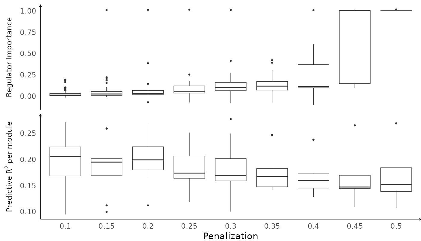

The results for each penalization parameter are placed in a list, results, attached to the fit object. So fit$results[[1]] contains the results of running scregclust with penalization = 0.1. For each penalization parameter, the algorithm might end up finding multiple optimal configurations. Each configuration describes target genes module assignments and which regulators are associated with which modules. The results for each such configuration are contained in the list output. This means that fit$results[[1]]$output[[1]] contains the results for the first final configuration. More than one may be available.

sapply(fit$results, function(r) length(r$output))
#> [1] 2 1 1 1 2 2 2 1 1

In this example, at most two final configurations were found for each penalization parameters.

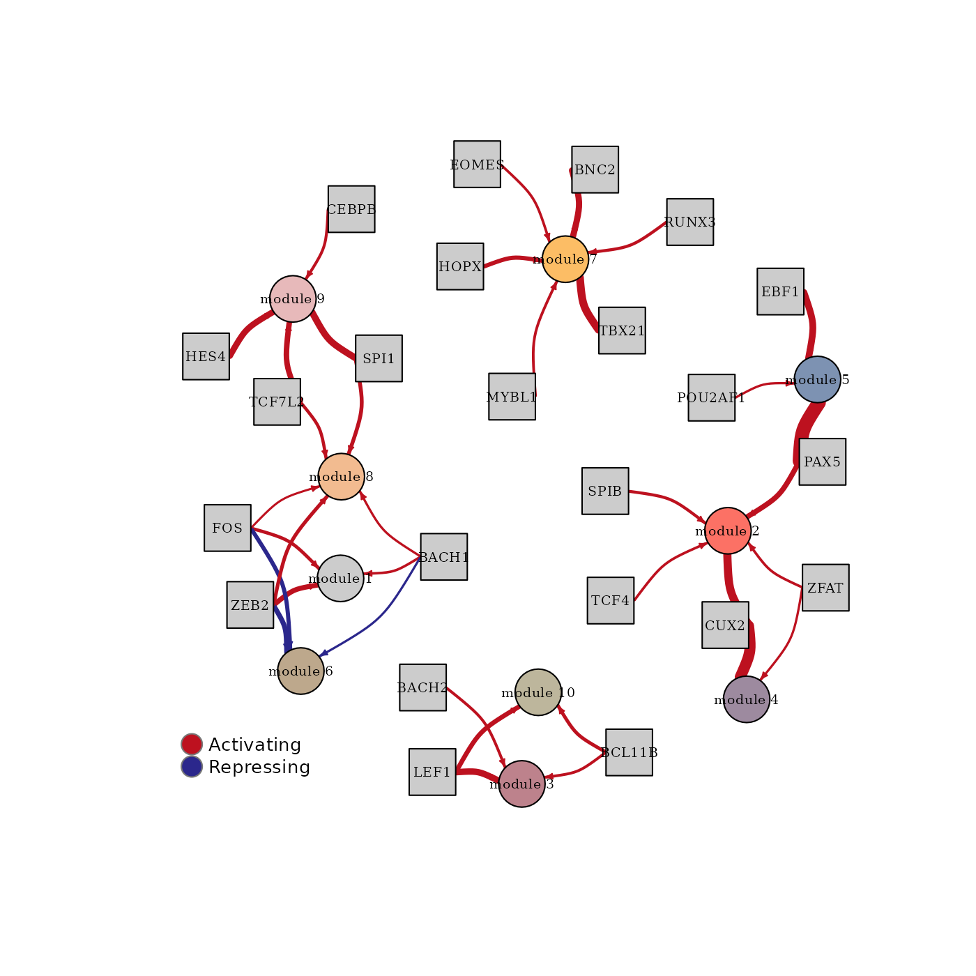
To plot the regulator network of the first configuration for penalization = 0.1 the function plot_regulator_network can be used.

plot_regulator_network(fit$results[[1]]$output[[1]])